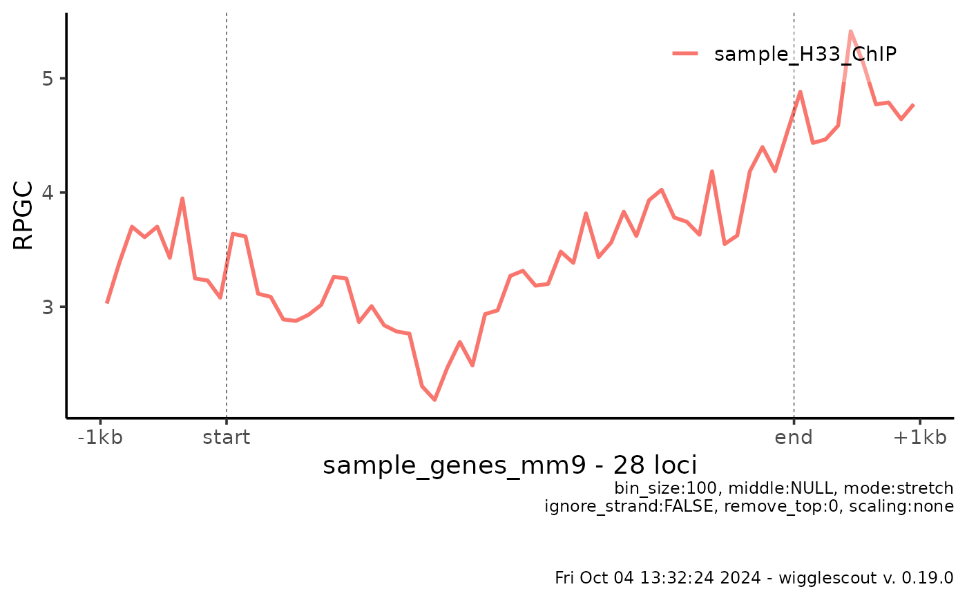
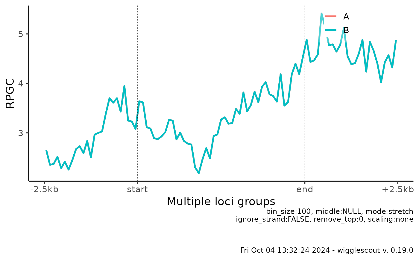
Plots a profile of a set of bigWig files over a set of loci in a BED file.
Usage
plot_bw_profile(
  bwfiles,
  loci,
  bg_bwfiles = NULL,
  mode = "stretch",
  bin_size = 100,
  upstream = 2500,
  downstream = 2500,
  middle = NULL,
  ignore_strand = FALSE,
  show_error = FALSE,
  norm_mode = "fc",
  labels = NULL,
  colors = NULL,
  remove_top = 0,
  verbose = TRUE,
  default_na = NA_real_,
  scaling = "none"
)
Arguments
- bwfiles
Path or array of paths to the bigWig files to be summarized.
- loci
BED file or GRanges to summarize
- bg_bwfiles
Path or array of paths to the bigWig files to be used as background.
- mode
How to handle differences in lengths across loci:
stretch: Anchor each locus on both sides.
start: Anchor all loci on start.
end: Anchor all loci on end.
center: Center all loci.
- bin_size
Bin size. Length of bin in base pairs. The lower, the higher the resolution.
- upstream
Number of base pairs to include upstream of loci.
- downstream
Number of base pairs to include downstream of loci.
- middle
Number of base pairs that the middle section has (in stretch mode). If not provided, median length of all loci is used.
- ignore_strand
Whether to use strand information in BED file.
- show_error
Show standard error.
- norm_mode
Function to apply to normalize bin values. Default fc: divides bw / bg. Alternative: log2fc: returns log2(bw/bg).
- labels
List of names to give to the mcols of the returned GRanges object. If NULL, file names are used.
- colors
Array of colors that will be assigned to labels or files (in that order)
- remove_top
Return range 0-(1-remove_top). By default returns the whole distribution (remove_top == 0).
- verbose
Put a caption with relevant parameters on the plot.
- default_na
Default value for missing values
- scaling
Whether to use the bigWig values as they are (none - default) or calculate relative enrichment (relative) by dividing values by global average.
Examples
# Get the raw files
bw <- system.file("extdata", "sample_H33_ChIP.bw", package="wigglescout")
bed <- system.file("extdata", "sample_genes_mm9.bed", package="wigglescout")


plot_bw_profile(bw, loci = bed,
                mode = "stretch", upstream = 1000, downstream = 1000)


# It is also possible to run same bigWig across several BED files or GRanges
plot_bw_profile(bw, loci = c(bed, bed), labels = c("A", "B"))
